Synth Lecture Notes DRAFT

Voltage as a sound analog

What is music from a physics perspective? Sound is variations in air pressure that excite the biomechanical systems in our ears. Musicians seek systems and instruments that can control air pressure variations in artistic ways. Humans have developed countless instruments to push the air in pleasing ways. To this day, the human voice remains our most fundamental and widely utilized instrument of air pressure manipulation. We can vary the frequency of those changes in air pressure (pitch), as well as the amplitude of the pressure variation (volume). When we vocalize, we don’t just produce a single pitch, but a spectrum of tones, each with varying amplitude. This variating spectrum of frequencies and amplitudes, which we can shape over time, gives each voice a signature quality (timbre). These characteristics (pitch, volume, timbre) apply to all the instruments we use in making music.

In the electronic age, the loudspeaker has become the primary air pressure manipulator. Music may still be initially created from non-electronic instruments, but the end result is broadcast across the internet and recreated by countless loudspeakers connected to personal computers (let’s include mobile phones in the “personal computer” category). Common loudspeaker systems are driven by power amplifiers that take voltage as input. The voltage is an analog for the sound pressure changes the musician wants their audience to experience.

A typical loudspeaker has two terminals, conventionally labeled + and -. These markings indicate which way the loudspeaker will move when a voltage is applied across the two terminals. It is conventional that when the applied voltage polarity matches the labels the speaker pushes outwards, and when the applied voltage is reversed the speaker pulls inwards.

The voltage driven loudspeaker system is the final goal whether the music was created purely by varying sound pressure (e.g. a microphone capturing a classical music performance), by varying voltage in electronic circuits (e.g. using a 1960s Moog synthesizer), or by storing sequences of data in digital files (e.g. MIDI files; digital audio workstations (DAWs)).

So what is voltage? Voltage is electrical pressure and is used as an analog for many physical quantities.

Voltage as signal

Every time a musician plugs in a 1/4-inch phone connector, they are tapping into a lineage of technology that dates back to the 1870s. This connector was the physical gateway to the first telephone networks: a system that did what the telegraph could not.

In the 19th century, high voltage sparks were used to send messages across vast distances. This was the technology of the telegraph, in which the presence or absence of a burst of electric energy could convey information, similar in spirit to our modern digital communications. However, such information was limited: while you could send a text message, you could not transmit your voice using a telegraph system. To make a telephone, we needed something that could modulate voltage smoothly with the human voice. Such a device is a microphone, and the first microphones, as used in telephones, were carbon microphones.

In a carbon microphone, the carbon material is placed in series with a battery and then the physical properties of the carbon are manipulated by the human voice. The varying sound pressure actuated a tiny mechanical system that clenched the carbon granules tighter as pressure increased, followed by loosening - a physical diffusion of the grains - when the pressure fell. The change in the density of the carbon was effectively a variable resistor: the resistance varies proportionally to nearby sound waves.

The carbon microphone was a very crude technology, but a good start. The telephone industry would refine this technology rapidly throughout the 20th century. The concept of the variable resistor component of the microphone led to the discovery of the electronic amplifier, realized initially with vacuum tubes and later with transistors. In all cases, the goal was to impress a small varying voltage onto a steady voltage. The small varying voltage we call the signal. Much of the science of using voltage as signals was discovered by the research lab of the American Telephone & Telegraph company (AT&T): Bell Labs. Bell Labs made music with computers in the 1950s.

Note on DSP

Digital effect plugins are an easy and potentially inexpensive (not counting the cost of the personal computer) way of learning about signal processing today. Mosts DAWs are bundled with a variety of effect plugins. While the signals are digital, the overall concept of processing the signals in series, parallel, or some combination of the two, is similar in both analog and digital form. The sequence of data that represents your music on a computer cannot be immediately transformed into varying sound pressure. There is always a digital-to-analog converter in series between your computer and the loudspeaker system (possibly multiple conversions).

Programmers think in terms of models when designing software. Digital audio software tends to use the language of analog systems, modelling these systems conceptually, not to be confused with physical modeling synthesis. In digital synthesis in particular, the models often reflect world of modular analog synthesizes quite closely. This is true in the Bell Labs MUSIC-N software all the way through its many descendants including the Web Audio API. This is all to say that is beneficial to study both analog and digital audio techniques.

Voltage as power (not signal)

This section describes voltages that are not signal voltages. In everyday life we usually need a power source specified with a nominal voltage (“120”, “5”, etc) to power our electronic lives. When you plug a cable into the wall, the wall is said to provide 120 volts, alternating current (ac). When you plug your phone charger into the wall, the wall provides 120 volts ac to the little box, and the little box provides 5 volts, direct current (dc) to your phone. We need to power our electronics, including amplifier systems, with a power source, and typically we are using the wall power or our power adapters with the assumption they will provide an infinite supply of energy for our system.

The alternating current in the wall happens to be sinusoidal, but we don’t consider it a signal. If you look at it on an oscilloscope, it will display as a sine wave at a fixed frequency. In the U.S., the frequency is usually 60 Hz. Musicians are frequently at odds with the noise the power lines make. If the 60 Hz sine wave was just an electromagnetic wave, we would not be able to hear it. Unfortunately, our audio amplifiers, driven by signal voltages, can not perfectly discriminate between our music and the power line “hum” of 60 Hz. The equal temperament system referenced to 440 Hz includes the frequencies 61.74 Hz and 58.27 Hz as “notes”, while 60 Hz is not considered a standard “note”. Therefore 60 Hz is generally an annoyance when it becomes audible.

Ultimately, we differentiate these voltages by their purpose: one provides energy, while the other carries information. A power voltage is intended to be a static, unchanging foundation: a “clean slate” that simply allows the device to turn on. Conversely, a signal voltage is defined by its changes; it is the dynamic waveform representing the music.

Oscillators

Electronic oscillators fall broadly into two categories: harmonic and relaxation.

Harmonic oscillators

Harmonic oscillators are sinusoidal and found in nature in many places. The story I like to tell goes like this: (note this really requires a live drawing of the cosine wave for the proper effect)

Imagine a playground with a swing set. You have a “bird’s-eye” view, directly overhead the swing set. I am standing a few feet away from the swing set, holding onto my child who is sitting in the swing. When I release my child, they build up speed due to gravity and go faster and faster, underneath the big pole, and climb upwards on the other side. As my child reaches their furthest distance from me, they slow to a brief halt, momentarily suspended in air, until gravity pulls them down and builds up speed to bring them back to me. If I provide a little push when my child returns to me, I can continue the action as long I have the energy and desire to do so.

The key moments to realize in the swing story are where my child is momentarily suspended in air. The swing momentarily comes to a complete stop whenever it changes direction. If you draw your “bird’s-eye” view of the pole and extend the pole to be a time axis, a trace of the swing’s journey over time is a trace of a cosine wave.

Non-electronic examples

Pause and consider various movement around you. If you pace back and forth across a room, can you instantaneously change direction when you reach a wall, or do you need to stop completely (if only briefly) in order to change direction? I suggest that most “natural” movement around us requires this rule of stopping, however briefly, and “smoothly” turning around, when we change directions. No teleportation is allowed the world we observe with the naked eye.

In a physics classroom, springs are often used as the prototypical harmonic oscillator. For musicians, an appropriate prototypical oscillator is the tuning fork.

Electronic examples

Musicians, especially those who perform using power amplification systems, have to contend with an occupational hazard: acoustic feedback. A microphone connected to a loudspeaker system may be disturbed by slight changes in air pressure, even in a quiet room. These small changes are then amplified by the loudspeaker (a dynamic speaker will move in and out the same way a dynamic microphone moves in and out), which may then appear as larger changes in air pressure for the microphone to receive and the process continues over and over until microphone and speaker create an audible tone that is loud, annoying, and potentially harmful. However, it is a good example of harmonic electronic (electro-acoustic) oscillator.

Similarly, those musicians who work in the recording studio may accidentally create a similar feedback loop using the extensive routing capabilities offered by recording equipment (e.g. a “mixer”, “console”, or “desk”). I encourage recording students to purposefully create these feedback paths on the analog equipment (with the loudspeakers turned to a minimum level) as a lab experiment. If the gain can be carefully controlled (the “channel fader” usually suffices), then just barely exceeding a system gain of +0 dB should generate a sine wave. EQ controls in the path provide a means to adjust the frequency of the oscillation.

Any amplifier system with positive gain can become an oscillator just by making the appropriate feedback connection.

Relaxation oscillators

Relaxation oscillators use a switching action to abruptly change their direction. A square wave is an example of a switched oscillation, and might even seem to be simpler than a sine wave, until you consider the practical implications of the ideal version. For an ideal square wave, the voltage level stays at its maximum output level for half its period, then instantaneously changes to the minimum output level for the other half of the period. Return to the story of my child on the swing set and imagine if my child’s motion was like an ideal square wave. Upon the release of my child, they would hover in place for several seconds, then abruptly appear hovering on the other side of the swing set for several seconds, then abruptly appear by be again. Clearly this is just a fantastical thought experiment, but doesn’t it drive home the idea of how unnatural such an oscillation is? In fact, real square wave oscillators do not abruptly switch from their maximum level to their minimum level, but simply move quickly enough that they appear to switch instantaneous for their application.

The more subtle thought experiment is the triangle wave: is that a plausible wave for a swing set to behave? The triangle doesn’t speed up and slow down to a halt like a sine wave. Rather it has a constant motion. I suggest if my child’s swinging motion matched a triangular wave, it would look like a bad animation of a child on a swing set. The motion would not match your intuition of what swinging looks like. Or imagine walking back and forth across a room at a constant speed: how could you possibly spin around and keep moving in the opposite direction without slowing down and speed up again?

Electronic example

This is a great circuit to breadboard. For those without knowledge of electronic circuits, consider the capacitor a “bucket” we are going to use to hold voltage. Using a battery, we can transfer the battery voltage to the capacitor. To slow down the transfer, we can use a resistor. To “dump the bucket out”, we can use a simple momentary switch. This arrangement gives us a simple oscillator, but we can easily improve it with two very useful features. The first is to straighten out the curve into a line. We can straighten the curve using a constant current source. We can make the switch automatic by replacing the mechanical switch with a transistor switch. The current source can be extended to allow for a control voltage input. The transistor switch can have it’s own input called hard sync.

Overtones, Harmonics

Gentle rocking a speaker back a forth with a sine wave triggers our ear to sense mostly one frequency. The hard blast of a square wave produces an acoustic wave that triggers many frequencies in our ear.

Filters

How does a low-pass filter distort square waves?

They can distort any wave into a sine wave. Note they do not distort sine waves.

Low-pass filters place a speed limit, or maximum, on the output signals.

(For those who know a little calculus, the low-pass filter is performing integration on the square wave.)

How does a high-pass filter distort square waves?

They distort square waves into impulses. The rising edges become positive pulses and the falling edges becomes negative pulses.

(For those who know a little calculus, the high-pass filter is performing differentiation on the square wave.)

Sawtooth waves will produce pulses in only one direction.

Given how radically the square and saw waves change, it is not unreasonable to guess that something interesting might happen to the sine waves, but sine waves pass without distortion, just attenuation.

One way to look at this is that high-pass filters place a sort of “speed minimum” on the output signals, as a dual to the speed limit enforced by the low-pass filters. The high-pass filter only reacts to (outputs) changing signals that are changing “fast enough” based on the parameter settings.

Filters as oscillators: the “resonance” control

If you cup your hands over your mouth to make an approximation of a tube to speak through, your voice becomes filtered. If you’re able to find other tubes around to speak through, you should notice a similar effect and the filtering changes with the physical dimensions of the tube. There are many musical instruments based on tuned tubes. If you blow air into them, they resonate.

With this idea that an electronic filter is analogous to a tuned tube, it shouldn’t be too hard to see that the blowing into the tube is similar to adding a positive feedback loop to the filter.

The sine waves produces by resonant filters in a synthesizer are usually good looking sine waves; better sine waves than those produced via wave-shaping in the VCO modules.

Control standards (1V/Oct) and historical context

Moog synthesizers are credited with popularizing the “1 volt-per-octave” standard, which was introduced with the Moog 901 oscillator in 1965.^{1 2} On the MOTM synthesizers and others, they may label jacks with “1V/OCT”, which can be quite cryptic for the uninitiated.

Showing the 1V/Oct keyboard output on the oscilloscope demystifies it. When played with no portamento (which is just low-pass filtering), the output resembles a typical MIDI note interface in a DAW. With the scope set to a vertical scale of 1V/division, the 1V/octave is easily verified.

Moog published two AES papers, both titled “Voltage-Controlled Electronic Music Modules”, in October 1964 and July 1965. These papers illustrate how Bob Moog approached the problem of making a musically useful oscillator. The basic idea of control voltage was not a novel idea, and Moog’s designs in the 1964 paper show an oscillator that has a control voltage input, but the voltage and frequency have a linear relationship: double the voltage and you double the frequency. By the next paper, Moog added two more circuits in front of his oscillator: a linear summation circuit (equivalent to an audio summing bus, but for control voltages to mix together), and an exponential converter that takes a linear input range and maps it to an exponentially changing frequency. No particular calibration is given in the AES paper, but that same year his 901 oscillator’s specification sheet states

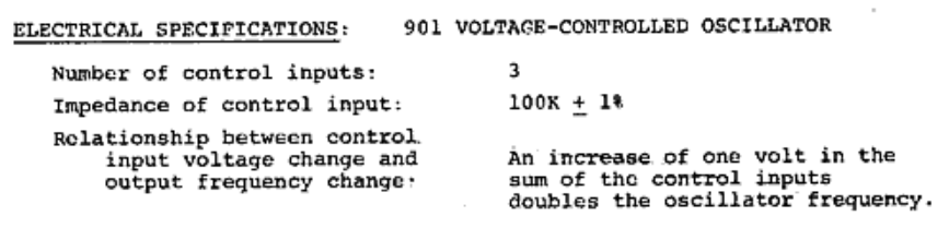
which solidified the 1 volt-per-octave standard.

Notable mention: Harald Bode

It is known that both Buchla and Moog were aware of Harald Bode’s work. Bode had an established career as an electronic musical instrument builder prior to 1960. In 1960, Bode presented the idea of a modular synthesizer at the AES convention. Bode did not describe voltage controlled oscillators, but he did describe an “envelope-shaping” system made from modular components. Herb Deutsch and Bob Moog were inspired by Harald Bode’s paper.³ Harald Bode would collaborate with Bob Moog and also worked for the Moog company.

Analog computers (optional)

Quote from Analog Days (p39):

Buchla’s familiarity with silicon transistors and his knowledge of analog computers (from working in physics) led him to voltage control …

Analog computers are of interest to understand the electronic landscape of the early 1960s from which both Buchla and Moog created very similar ideas independently. The operational amplifier, or “op-amp”, was developed for analog computers. Operation here refers to the arithmetic operations of addition, subtraction, multiplication, and division. In audio you add and subtract when you mix your signals together on a DAW or console. When you you use a fader, you are multiplying (+dB) or dividing (-dB) your signal by a constant coefficient proportional to the position of the fader.

Users of analog computers did not create sound, but they did create waveforms to view on oscilloscopes and plotters (devices similar to a printer) to solve math problems. In order to solve a problem, equations are written down and translated into patches on an analog computer, just like how you patch a modular synthesizer. Analog synthesizers are arguably a specialized analog computer. There are many types of specialized analog computers (see page 10 of EAI Handbook of Analog Computation, 1967).

Test equipment (optional)

Another place to examine for historical context is 1950s and 1960s test equipment. This is equipment both Buchla and Moog would have used at school, and would have to own in their shops to test their creations and try new ideas.

Different specification example (optional)

What other standards might have worked?

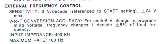
Here’s a link to a 1968 journal that has the HP Model 3305A Sweep Plug-In specifications. The specifications say:

EXTERNAL FREQUENCY CONTROL

SENSITIVITY: 6 V/decade +/-24 V max.

V-to-F CONVERSION ACCURACY: For each 6 V change in programming voltage, frequency changes 1 decade +/-5% of final frequency.

Specific synthesizer notes

This is just a random collection of notes pertaining to hardware synths that were typically available during the lecture.

MOTM modular system

Patch: Sample & Hold

More of a demo note: it’s fun to display the noise source on the scope, then pause the scope and zoom in to see that the noise has a continuous value and is smoothly curved.

The MOTM Sample and Hold includes a sample input jack so I sample a triangle LFO and display both the source and sampled output simultaneously on two scope channels.

Roland Juno 60

Roland called the Juno oscillators “digitally controlled oscillators” or DCOs. The oscillators are still analog, relaxation oscillator circuits that create a sawtooth core waveform and derive the other options from that core. The initial frequencies of all six oscillators are under the control of the microcontroller (8049 type) (by initial I mean without other CV inputs like the bender or LFO). The microcontroller outputs an 8-bit word that goes through a discrete R-2R ladder digital-to-analog converter (DAC).

Patch: Monophonic mode

You can put the Juno 60 in monophonic mode (all six oscillators play in unison) by powering it on with the transpose button held and then putting the arp mode in the “up” position. Viewing the monophonic output on an oscilloscope, the waveforms align perfectly, and the sound lacks the slow beating that six free-running VCOs would have.

The chorus circuit was allegedly included to thicken the sound as two-oscillators per voice was considered a “standard” in subtractive synthesis and the Juno only assigned one oscillator per voice. Using the sub-octave waveform, which is just a simple divide-by-two of the core oscillation, has the same issue the phase locked mono output has: it lacks the natural beating/chorusing that two free-running oscillators would have.

Moog Minimoog

Patch: Ext Input Feedback Loop

• Patch the main output into the external input and turn the input on and up all the way.
• Leave the resonance all the way off.
• Slowly sweep the filter or use the amplifier envelope to create long, slow envelopes.

Moog Rogue

Patch: Hard Sync Sweep

I love a hard sync sweep patch, and the Moog Rogue makes it really easy.

• In OSCILLATORS, set SYNC to CONTOURED
• Use the OCTAVE switch and INTERVAL control to set the initial conditions
• Use the CONTOUR GENERATOR ATTACK and DECAY sliders to set the time constants
• Use the FILTER AMT slider to adjust the effect when triggered

Notes on the notes

This is a written version of a lecture I have given at the Clive Davis Institute of Recorded Music for many years. The lecture began as a demonstration of a small MOTM modular system with an oscilloscope. In the beginning I thought students might like to hear unusual patches, but that approach I found unsatisfactory.

One problem was the time spent patching: it is quite boring for the audience to watch you patch. Trying to talk and patch at the same time is quite difficult. If possible I just say what I’m doing (“now I’m connecting the oscillator sawtooth output to the …”) which gets hard to follow if the patch is too complex.

Another issue was that patches that wowed one crowd might bomb with another. So I moved “prepared patches” to the very start, assuming I had time to patch before the start. If the patch were a hit, maybe it would generate some good comments or questions to support the lecture, and if the patch was a dud I didn’t need to comment on it.

Questions usually were along the lines of “what is an oscillator?” or “when does the oscillator turn-on?” rather than “how do get an X sound?”

The oscilloscope ended up being the star of the show. Using the scope separated this demo from all the other synth demos they had experienced before. Unfortunately, I found many students didn’t really understand what information they were supposed to get from the waveforms on the oscilloscope screen. I realized I would have to define what a voltage is and motivate why a musician would care about voltage by discussing loudspeakers and microphones (after revisiting Moog manuals, I found they had a similar approach - see the Moog Rogue manual for instance).

The intended audience for this lecture is assumed to have a strong music background, but no higher level math or science knowledge. My goal is to expose this audience to some insights I gained into electronic music as a musician, synthesizer technician, and electrical engineer - in that order.